Probability Basics
Based on the article “A Barebones Guide to Mechanistic Interpretability Prerequisites” written by Neel Nanda
Basics of distributions : expected value, standard deviation, normal distributions
To a 5-year old
Imagine you have a bag of candies, and you’re going to share them with your friends.
Expected Value (Average Share): If you know how many candies are in the bag and how many friends you have, the “expected value” is like figuring out how many candies each friend would get if you shared them out evenly. It’s the fair share, the average amount.
Standard Deviation (How Spread Out the Shares Are): Now, maybe you don’t share them perfectly evenly. Some friends might get a few more, and some might get a few less. The “standard deviation” tells you how much the shares are different from that even share. A small standard deviation means everyone got about the same amount. A big standard deviation means some got a lot more, and some got a lot less.
Normal Distribution (The Most Common Way): Imagine if you did this candy sharing game many, many times. Most of the time, the shares would be somewhere in the middle, close to that even amount. Sometimes, a few friends might get a lot more or a lot less, but that wouldn’t happen as often. The “normal distribution” is like saying that most of the results will be around the average, and fewer results will be far away from the average, making a nice bell shape if you drew a picture of it. It’s like most kids are of average height, and only a few are very tall or very short.
1
2
3
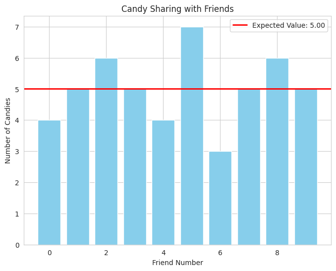
- We simulate candy sharing with a list of how many candies each friend got.
- We calculate the expected value (average).
- The bar plot shows each friend's share, and the red line shows the average. This visually represents the "fair share," and how individual shares deviate from it.
To an ungergraduate student
Let \(X\) be a random variable with a probability distribution \(P(x)\).
- Expected Value (\(E[X]\) or \(μ\)): The expected value is the long-run average value of \(X\). For a discrete distribution, it’s: \(E[X]=∑xP(x)\) For a continuous distribution with probability density function (PDF) \(f(x)\), it’s: \(E[X]=\int_{-\infty}^{\infty} xf(x)dx\) It represents the central tendency or the mean of the distribution.
- Standard Deviation (\(σ\)): The standard deviation measures the dispersion or spread of the distribution around its mean. It’s the square root of the variance \((Var(X))\): \(Var(X)=E[(X−μ)^2]=E[X^2]−(E[X])^2\) \(σ=\sqrt{Var(X)}\) A small standard deviation indicates that the values of \(X\) are clustered closely around the mean, while a large standard deviation indicates a wider spread.
Normal Distribution (Gaussian Distribution): The normal distribution is a continuous probability distribution characterized by its bell-shaped PDF: \(f(x∣μ,σ^2)=\frac{1}{\sqrt{2πσ^2}}e^{-\frac{(x−μ)^2}{2σ^2}}\) where \(μ\) is the mean (expected value) and \(σ^2\) is the variance. Key properties of the normal distribution:
- It’s symmetric around the mean.
- The mean, median, and mode are all equal.
- Approximately 68% of the data falls within one standard deviation of the mean \((μ±σ)\).
- Approximately 95% of the data falls within two standard deviations of the mean \((μ±2σ)\).
- Approximately 99.7% of the data falls within three standard deviations of the mean \((μ±3σ)\). The normal distribution arises naturally in many situations due to the Central Limit Theorem, which states that the sum (or average) of a large number of independent, identically distributed random variables will approximately follow a normal distribution, regardless of the original distribution.
1
2
3
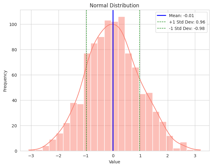
- We generate data from a standard normal distribution (mean 0, standard deviation 1).
- The histogram shows the bell shape of the normal distribution.
- The blue line indicates the mean (expected value), and the green dashed lines show one standard deviation away from the mean, illustrating the spread of the data.
To an AI/ML engineer
Understanding distributions is fundamental in AI/ML for data analysis, model selection, and probabilistic reasoning.
Expected Value: In ML, the expected value can represent the average prediction of a model over many instances, the average value of a feature in a dataset, or the long-term average reward in reinforcement learning. It’s a crucial measure of the central tendency of data or model outputs.
Standard Deviation: The standard deviation quantifies the uncertainty or variability in data or model predictions. A high standard deviation in model outputs might indicate instability or high variance. In feature analysis, it helps understand the spread of values for each feature. It’s also used in normalization techniques to scale features to a similar range.
Normal Distribution: The normal distribution is a ubiquitous assumption in many statistical models and ML algorithms due to its mathematical tractability and the Central Limit Theorem.
- Modeling Errors: Often, the error terms in regression models are assumed to be normally distributed.
- Feature Distribution: Some feature scaling techniques assume or aim for a roughly normal distribution.
- Probabilistic Models: Gaussian processes, Gaussian mixture models, and many Bayesian methods heavily rely on the properties of normal distributions.
- Initialization: Weights in neural networks are often initialized from normal distributions.
- Anomaly Detection: Deviations from a normal distribution can be indicative of anomalies.
However, it’s crucial to remember that real-world data is not always normally distributed. Understanding the actual distribution of data is essential for choosing appropriate models and avoiding incorrect assumptions. Techniques for assessing normality (e.g., visual inspection, statistical tests) and handling non-normal data (e.g., transformations, non-parametric methods) are important.
Furthermore, in deep learning, while individual weights might be initialized normally, the distributions of activations and learned representations can be complex and non-Gaussian. Understanding these learned distributions is an active area of research.
1
2
3
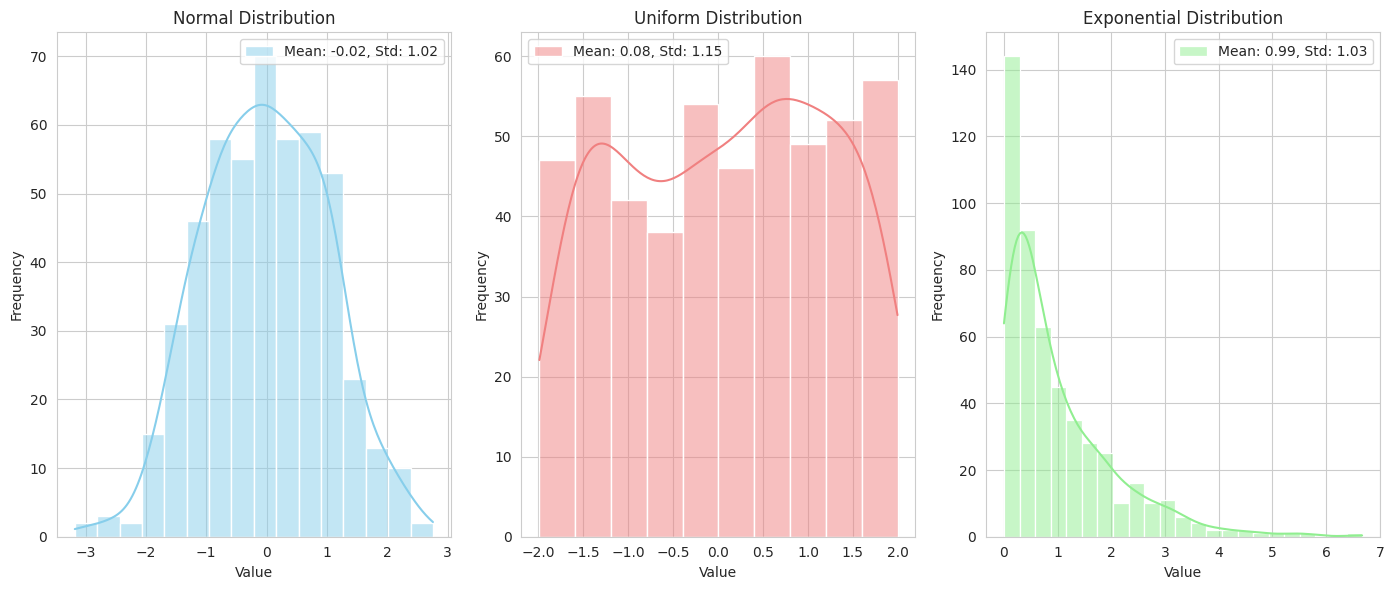
- We generate data from three different distributions: normal, uniform, and exponential.
- We plot histograms of each distribution with kernel density estimates (KDEs) to visualize their shapes.
- The mean and standard deviation are printed in the legend for each distribution. This highlights that different distributions have different shapes and are characterized by their expected value and standard deviation, which is crucial for choosing appropriate models and understanding data in AI/ML.
Log likelihood
To a 5-year old:
Imagine you have a bag with some red and blue balls, but you don’t know exactly how many of each color. Your friend takes out a ball, shows you it, and puts it back. They do this many times.
Likelihood (How Likely Your Guess is): Every time your friend shows you a ball, you can make a guess about how many red and blue balls are in the bag. If you see mostly red balls, you might guess there are many more red balls than blue balls. The “likelihood” is like how much your guess makes sense based on the balls you’ve seen. If you guessed mostly blue balls and you keep seeing red, the likelihood of your guess is low.
Log Likelihood (Making it Easier to Work With): The “log likelihood” is just a special way to keep track of how good your guesses are. It’s like using a special number system that makes it easier to compare how likely different guesses are, especially when you see many balls in a row. Instead of multiplying how likely each guess was for each ball, you add them up. Adding is easier than multiplying when you have many numbers! A bigger “log likelihood” number means your guess is more likely to be right.
So, when you’re guessing the colors in the bag, the log likelihood helps you find the best guess that fits the balls you’ve seen so far, by making it easier to keep track of how well each guess matches the evidence.
1
2
3
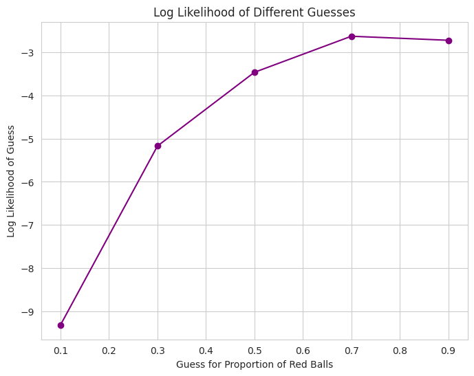
- We simulate a guessing game with red and blue balls.
- We calculate the log likelihood of different guesses for the proportion of red balls given a sequence of observations.
- The plot shows how the log likelihood changes with different guesses. The peak of the curve would represent the most likely guess.
To an undergraduat student:
In statistics and machine learning, we often want to estimate the parameters $θ$ of a probability distribution $P(x∣θ)$ given a set of observed data $X={x_1,x_2,…,x_n}$.
Likelihood Function $(L(θ∣X))$: The likelihood function is the probability of observing the data $X$ given a particular set of parameters $θ$. Assuming the data points are independent and identically distributed (i.i.d.), the likelihood is the product of the probabilities (or probability densities for continuous data) of each data point: \(L(θ∣X)=P(X∣θ)=∏_{i=1}^{n}P(x_{i}∣θ)\) The likelihood function tells us how plausible different values of $θ$ are, given the observed data $X$. A higher likelihood value indicates that the parameters $θ$ make the observed data more probable.
Log Likelihood $(ℓ(θ∣X))$: Working with the product of probabilities can be mathematically inconvenient (e.g., prone to underflow for large $n$). The log likelihood is the natural logarithm of the likelihood function: \(ℓ(θ∣X)=logL(θ∣X)=log(∏_{i=1}^{n}P(x_i∣θ))=∑_{i=1}^{n}logP(x_i∣θ)\)Taking the logarithm transforms the product into a sum, which is often easier to work with for optimization and analytical purposes. Since the logarithm is a monotonic function, maximizing the log likelihood is equivalent to maximizing the likelihood.
Why is Log Likelihood useful?
Mathematical Convenience: Sums are generally easier to differentiate and optimize than products. Many parameter estimation techniques (like Maximum Likelihood Estimation - MLE) involve finding the parameters $θ$ that maximize the (log) likelihood function by taking derivatives and setting them to zero.
Numerical Stability: Multiplying many small probabilities can lead to very small numbers (underflow). Summing the logarithms of these probabilities keeps the numbers in a more manageable range.
Information Interpretation: The log likelihood can be related to information theory concepts. For example, the negative log likelihood is related to the cross-entropy between the model’s predicted distribution and the empirical distribution of the data.
Properties of Logarithm: The logarithm function has useful properties (e.g., $log(ab)=loga+logb$) that simplify calculations and derivations.
1
2
3
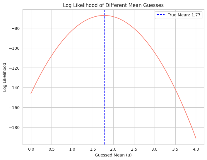
- We generate sample data from a normal distribution with a known mean.
- We calculate the log likelihood of the data under different assumed means (while keeping the standard deviation fixed).
- The plot shows that the log likelihood is maximized when the guessed mean is close to the true mean of the data. This illustrates the principle of maximum likelihood estimation.
To an AI/ML engineer
The log likelihood plays a central role in training probabilistic models and evaluating their performance.
Model Training (Maximum Likelihood Estimation): Many machine learning models with probabilistic interpretations are trained by maximizing the log likelihood of the training data given the model’s parameters $θ$. This is the principle behind Maximum Likelihood Estimation (MLE). The goal is to find the parameter values that make the observed training data most probable under the model’s assumed distribution. Examples include:
- Logistic Regression: The model parameters (weights) are often learned by maximizing the log likelihood of the binary labels given the input features.
- Naive Bayes: The class probabilities and feature conditional probabilities are estimated by maximizing the log likelihood of the training data.
- Neural Networks (with probabilistic outputs): When a neural network outputs probabilities (e.g., through a softmax layer for classification), the model is often trained using a loss function that is directly related to the negative log likelihood (like cross-entropy).
Loss Functions: Many common loss functions in AI/ML are derived from the negative log likelihood. Minimizing the negative log likelihood is equivalent to maximizing the log likelihood. For example, the cross-entropy loss for classification is the negative log likelihood of the true class labels under the model’s predicted probability distribution.
Model Evaluation: The log likelihood (or related metrics like perplexity, which is related to the exponential of the negative log likelihood) can be used to evaluate how well a probabilistic model fits the observed data. A higher log likelihood on unseen data (test set) generally indicates a better model.
Bayesian Inference: In Bayesian methods, the log likelihood of the data given the parameters is a key component in Bayes’ theorem, which combines the prior belief about the parameters with the evidence from the data to obtain the posterior distribution of the parameters.
Generative Models: In generative models (e.g., Variational Autoencoders - VAEs, Generative Adversarial Networks - GANs), the log likelihood (or a tractable lower bound on it) is often a key objective function to optimize during training.
1
2
3
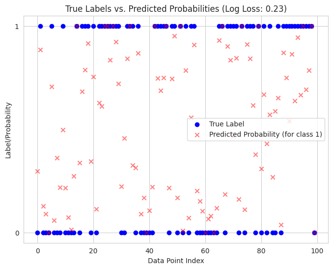
- We simulate a binary classification scenario with true labels and predicted probabilities from a hypothetical model.
- We calculate the log loss, which is the negative log likelihood used as a loss function in logistic regression and other classification models.
- We visualize the true labels and the predicted probabilities. The log loss value indicates how well the model's probabilistic predictions align with the actual outcomes. Lower log loss signifies better performance.
Maximum value estimators
To a 5-year old
Imagine you have a box of toys that were made by either Toy Maker A or Toy Maker B. You don’t know which one made them.
Your Goal: You want to guess who made the toys.
How You Guess: You look closely at the toys. Maybe Toy Maker A usually makes cars with square wheels, and Toy Maker B usually makes cars with round wheels. If you see a lot of cars with round wheels in your box, you’d probably guess that Toy Maker B made them.
Maximum Likelihood Estimator (The Best Guesser): The “Maximum Likelihood Estimator” is like the smartest person who looks at all the toys and makes the best guess about who made them. They choose the toy maker (the “parameter” we’re guessing) that makes the toys you see the most likely. If seeing round wheels is very likely if Toy Maker B made them, then Toy Maker B is their best guess.
So, the MLE is the guess that makes the things you’ve seen the most probable.
1
2
3
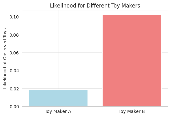
- We have a simple scenario of guessing between two toy makers based on observed toys.
- We calculate the likelihood of seeing the observed toys if each toy maker was responsible.
- The bar plot visually compares these likelihoods, showing which toy maker is the "maximum likelihood estimator."
To an undergraduate student
In statistics, we often want to estimate the parameters $θ$ of a probability distribution that best explains a set of observed data $X={x_1,x_2,…,x_n}$.
- Likelihood Function ($L(θ∣X)$): As we discussed before, the likelihood function is the probability of observing the data $X$ given a particular set of parameters $θ$: (for i.i.d. data)\(L(θ∣X)=P(X∣θ)=∏_{i=1}^{n}P(x_i∣θ)\)
Maximum Likelihood Estimator ($\hat{θ}_{MLE}$): The Maximum Likelihood Estimator (MLE) of the parameter $θ$ is the value $\hat{θ}$ that maximizes the likelihood function: \(\hat{θ}_{MLE}=argmax_θL(θ∣X)\) In other words, the MLE is the parameter value that makes the observed data $X$ most probable under the assumed probability distribution.
- Log Likelihood (Practical Optimization): As mentioned earlier, it’s often easier to work with the log likelihood: \(ℓ(θ∣X)=logL(θ∣X)=∑_{i=1}^{n}logP(x_i∣θ)\) Maximizing the log likelihood is equivalent to maximizing the likelihood, and the MLE is often found by solving: \(\frac{d}{dθ}ℓ(θ∣X)=0\) (or gradient is zero for multi-parameter cases)
Why is MLE useful?
Intuitive Interpretation: MLE aims to find the parameters that best “fit” the observed data in a probabilistic sense.
Asymptotic Properties: Under certain regularity conditions, MLEs have desirable asymptotic properties (as the sample size n becomes large):
- Consistency: The MLE converges to the true parameter value.
- Asymptotic Normality: The distribution of the MLE approaches a normal distribution.
- Efficiency: The MLE achieves the Cramer-Rao lower bound for variance, meaning it’s asymptotically the minimum variance unbiased estimator.
Widely Applicable: MLE is a fundamental technique used in a vast range of statistical models and machine learning algorithms for parameter estimation.
1
2
3
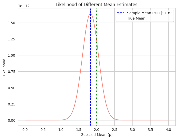
- We generate data from a normal distribution with a known true mean.
- We calculate the likelihood of the data for a range of possible mean estimates.
- The plot shows how the likelihood changes as we vary our guess for the mean. The peak of the curve occurs at the sample mean, which is the MLE for the mean of a normal distribution.
To an AI/ML engineer
Maximum Likelihood Estimation (MLE) is a core principle behind many learning algorithms, especially for probabilistic models.
Model Parameter Learning: When training a model with parameters $θ$ to fit data $X$, if the model provides a probability distribution $P(X∣θ)$ over the data (or the labels given the data), MLE aims to find the parameter values $\hat{θ}$ that maximize the probability of observing the training data.
Loss Functions as Negative Log Likelihood: Many common loss functions in AI/ML are directly derived from the negative log likelihood. Minimizing these loss functions is equivalent to maximizing the log likelihood. Examples include:
- Cross-entropy loss in classification: For a categorical distribution over classes, minimizing cross-entropy is equivalent to maximizing the log likelihood of the true class labels.
- Mean Squared Error (MSE) in regression (under Gaussian noise assumption): If we assume the target variable is normally distributed around the model’s prediction with constant variance, minimizing MSE is equivalent to maximizing the log likelihood.
Training Probabilistic Models: MLE is fundamental for training models that output probabilities, such as:
- Logistic Regression: Learns weights by maximizing the log likelihood of the binary labels.
- Naive Bayes: Estimates probabilities by maximizing the log likelihood of the features given the class and the prior class probabilities.
- Gaussian Mixture Models (GMMs): Learns the parameters of the Gaussian components by maximizing the log likelihood of the data.
Limitations: MLE can be prone to overfitting, especially with small datasets and complex models, as it tries to perfectly fit the training data, including noise. Regularization techniques are often used in conjunction with MLE to mitigate this.
Bayesian Perspective: In contrast to MLE, which finds a point estimate for the parameters, Bayesian methods aim to find the entire posterior distribution of the parameters given the data and a prior distribution, using Bayes’ theorem. The likelihood function (which MLE maximizes) is a key component in Bayesian inference as well.
1
2
3
4
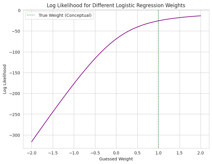
- We create a simplified conceptual example of MLE in logistic regression.
- We simulate binary data and consider a logistic model with a single weight parameter we want to estimate.
- We calculate the log likelihood of the true labels for different possible values of this weight.
- The plot shows how the log likelihood changes with the weight. The MLE would be the weight value at the peak of this curve, representing the weight that makes the observed labels most probable under the logistic model.
Random variables
To a 5-year old
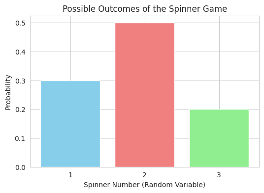
Imagine you’re playing a game where you spin a spinner with different numbers on it (like 1, 2, 3).
The Game’s Outcome: Each time you spin, you get a number. That number is the surprise result of your spin.
Random Variable (The Label for the Surprise): A “random variable” is just a fancy name for something that can have different surprise outcomes, and you don’t know exactly what it will be until you play the game (spin the spinner). We can give it a name, like “The Spinner Number.”
Different Surprises: “The Spinner Number” can be 1, or 2, or 3. These are the different possible values of our random variable.
So, a random variable is like the label for the surprise result of a game where you don’t know what will happen until you play!
1
2
-   We simulate a spinner game where the outcome (the number) is a random variable.
-   A bar plot shows the possible outcomes and their associated probabilities, illustrating that the random variable can take different values with different likelihoods.
To an undergraduate student
In probability theory, a random variable is a function that maps the outcomes of a random experiment (from a sample space $Ω$) to real numbers (or sometimes to vectors or other mathematical objects).
Let $(Ω,F,P)$ be a probability space, where:
- $Ω$ is the sample space (the set of all possible outcomes).
- $F$ is a sigma-algebra on $Ω$ (a collection of subsets of $Ω$ representing events).
- $P$ is a probability measure on $(Ω,F)$.
A random variable $X$ is a function $X:Ω→R$ such that for every real number $x$, the set ${ω∈Ω∣X(ω)≤x}$ (the event that $X$ takes a value less than or equal to $x$) is in the sigma-algebra $F$. This condition ensures that we can assign probabilities to events defined in terms of the random variable.
Types of Random Variables:
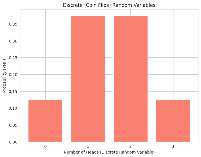
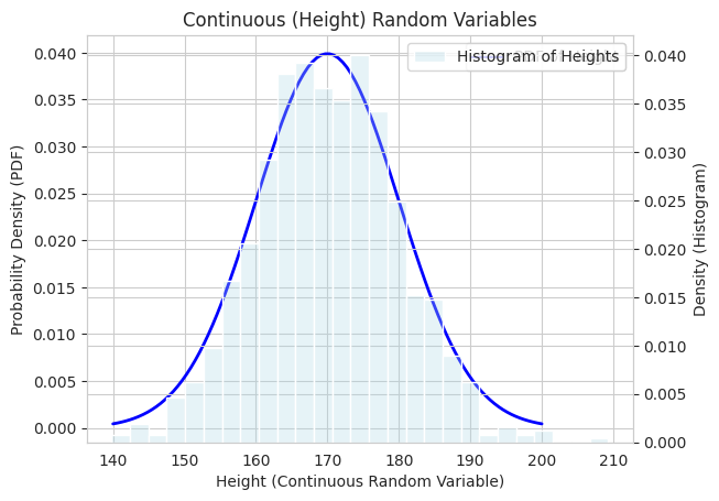
- Discrete Random Variable: Can take on a countable number of distinct values (e.g., the number of heads in 10 coin flips, the number rolled on a die). Its probability distribution is described by a probability mass function (PMF).
- Continuous Random Variable: Can take on any value within a continuous range (e.g., height of a person, temperature). Its probability distribution is described by a probability density function (PDF).
What do random variables allow us to do?
- Quantify Randomness: They provide a way to assign numerical values to the outcomes of random experiments.
- Study Probability Distributions: We can analyze the probabilities associated with different values or ranges of values that a random variable can take.
- Calculate Statistical Measures: We can compute quantities like the expected value, variance, and standard deviation of a random variable.
- Build Mathematical Models: They are fundamental building blocks for constructing probabilistic models of real-world phenomena.
1
2
-   We demonstrate both a discrete random variable (number of heads in coin flips) with its Probability Mass Function (PMF) shown as a bar plot.
-   We also show a continuous random variable (height) by simulating data from a normal distribution and plotting its Probability Density Function (PDF) as a line, along with a histogram to show the distribution of the sampled values.
To an AI/ML engineer
Random variables are essential for representing data, modeling uncertainty, and building probabilistic models.
Data as Realizations of Random Variables: Each feature in a dataset can be viewed as a realization of a random variable. For example, the height of a person in a dataset is one observed value from the random variable “Height.” Understanding the distribution of these random variables (features) is crucial for data analysis and preprocessing.
Modeling Uncertainty: Random variables are used to model the inherent randomness or uncertainty in various aspects of AI/ML:
- Noise in data: Measurement errors or random fluctuations can be modeled using random variables.
- Model parameters (in Bayesian methods): In Bayesian inference, model parameters are treated as random variables with probability distributions.
- Predictions: Probabilistic models output predictions in the form of probability distributions over possible outcomes, essentially defining a random variable for the prediction.
Probabilistic Models: Many AI/ML models are inherently probabilistic and rely heavily on the concept of random variables:
- Generative Models (e.g., GANs, VAEs): These models learn the underlying probability distribution of the training data, allowing them to generate new samples from that distribution. The generated data points are realizations of the learned random variables.
- Bayesian Networks: These are graphical models that represent probabilistic relationships between a set of random variables.
- Hidden Markov Models (HMMs): These models use hidden random variables to model sequential data.
- Reinforcement Learning: The state, action, and reward in an RL environment can often be modeled as random variables.
Statistical Inference: Random variables are the foundation for statistical inference in AI/ML, allowing us to draw conclusions about populations based on samples (e.g., hypothesis testing, confidence intervals).
Model Evaluation: Metrics like log-likelihood evaluate how well a model’s predicted probability distribution (over a random variable) matches the observed data.
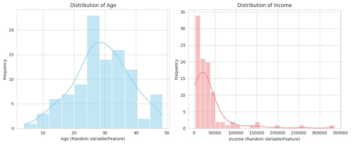
1
2
-   We simulate two common types of features in datasets: Age (which might be approximately normally distributed) and Income (which often has a skewed distribution like log-normal).
-   Histograms with Kernel Density Estimates (KDEs) are plotted for each feature. This illustrates how features in a dataset can be viewed as realizations of random variables with specific distributions, which is crucial for tasks like feature engineering and model selection.
Central limit theorem
To a 5-year old:
Imagine you have lots and lots of bags filled with marbles. Each bag has a different mix of red, blue, and green marbles.
Taking a Peek: If you just look at one bag, you might see mostly red, or mostly blue, or a mix. The number of each color in one bag can be all sorts of different.
Counting the Average: Now, what if you take just a few marbles out of each bag and count how many red ones you picked in total from all those bags? Then you do this again and again, each time taking a few marbles from every single bag.
The Magic: Even though each bag was different, if you do this “taking a few from each and counting the total” many, many times, the number of red marbles you get in total each time will start to follow a very special pattern. It will look like a nice, smooth hill shape (like the normal distribution we talked about before).
The Central Limit Theorem is like saying that if you take a little bit from many different things and add them up, the total will often follow this nice hill shape, no matter what the original things looked like!
1
2
3
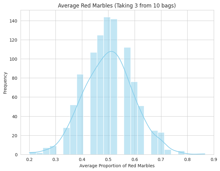
- We simulate drawing marbles (representing a binary outcome) from multiple "bags" with different mixes.
- We calculate the average proportion of red marbles drawn across all bags in each simulation.
- The histogram shows the distribution of these averages over many simulations. You'll see a tendency towards a bell shape, illustrating the CLT in a simple context.
To an undergraduate student
The Central Limit Theorem (CLT) is a fundamental concept in probability theory. It states that the distribution of the sample mean (or sum) of a large number of independent, identically distributed (i.i.d.) random variables will be approximately normally distributed, regardless of the shape of the original distribution.
More formally:
Let $X_1,X_2,…,X_n$ be a sequence of $n$ i.i.d. random variables with mean $μ$ and finite variance $σ^2$. Let $\bar{X}n=\frac{1}{n}∑{i=1}^{n}X_i$ be the sample mean.
Then, as $n→∞$, the distribution of the standardized sample mean: \(Z_n=\frac{\bar{X}_n−μ}{σ/\sqrt{n}}\) converges in distribution to a standard normal distribution $N(0,1)$.
Similarly, the distribution of the sample sum $S_n=∑_{i=1}^{n}X_i$ converges to a normal distribution with mean $nμ$ and variance $nσ^2$, i.e., $N(nμ,nσ^2)$.
Key Implications:
- Normality of Sample Means: Even if the original population distribution is not normal (e.g., uniform, exponential, binomial), the distribution of the sample mean will tend towards normality as the sample size n increases.
- Approximation for Large Samples: For sufficiently large n (often n≥30 is used as a rule of thumb, but it depends on the skewness of the original distribution), we can use the normal distribution to approximate the distribution of sample means and sums.
- Foundation for Statistical Inference: The CLT is crucial for many statistical inference procedures, such as hypothesis testing and confidence interval construction, as they often rely on the assumption of normally distributed sample statistics.
1
2
3
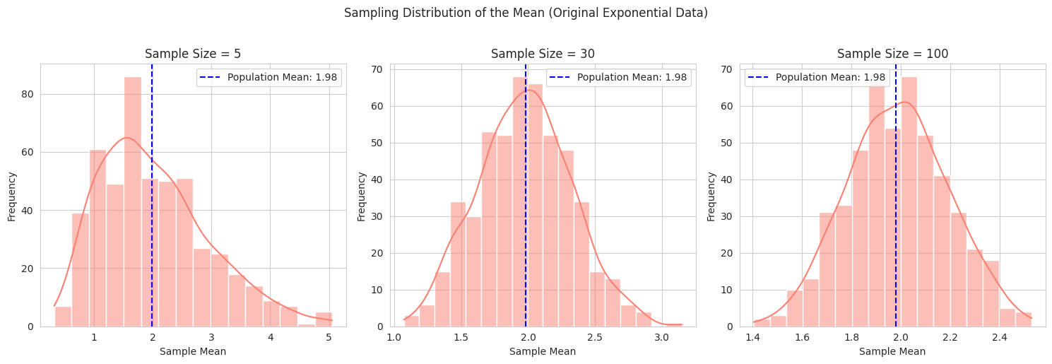
- We start with data from a non-normal distribution (exponential).
- We then repeatedly take random samples of different sizes from this original data and calculate the mean of each sample.
- We plot the distribution of these sample means for increasing sample sizes. The visualization clearly shows how the distribution of the sample means becomes increasingly normal and more tightly centered around the true population mean as the sample size grows.
To an AI/ML Engineer
The Central Limit Theorem (CLT) has significant implications in AI/ML, particularly when dealing with data aggregation and understanding the behavior of certain algorithms.
Feature Engineering and Aggregation: When creating new features by averaging or summing multiple independent features, the CLT suggests that the distribution of these new features will tend towards a normal distribution as the number of aggregated features increases. This can be useful for simplifying feature distributions or making them more amenable to certain models that assume normality.
Understanding Model Behavior:
- Ensemble Methods: Techniques like Bagging (Bootstrap Aggregating) involve averaging predictions from multiple models trained on different subsets of the data. The CLT provides a theoretical basis for why the aggregated prediction often has lower variance and can be more robust, as the average of many (somewhat) independent model outputs tends towards a more stable distribution.
- Gradient Estimation in Stochastic Optimization: In training large-scale models with stochastic gradient descent (SGD), the gradient is estimated based on a small batch of data. The CLT suggests that as the batch size increases, the distribution of the estimated gradient will become more normally distributed around the true gradient, which can influence the convergence properties of the optimization algorithm.
Statistical Inference on Model Performance: When evaluating model performance using metrics calculated on a test set (which can be seen as a sample of predictions), the CLT can be invoked to make inferences about the distribution of these metrics (e.g., the mean squared error or accuracy) if the test set is large enough and the individual errors or outcomes are reasonably independent. This allows for constructing confidence intervals for performance estimates.
Assumptions in Statistical Models: While the CLT is powerful, it’s important to remember that many statistical models in AI/ML explicitly assume normally distributed data or residuals. The CLT provides some justification for this assumption when dealing with aggregated quantities or large samples, but it doesn’t guarantee normality for the original data itself. It’s crucial to validate these assumptions.
Bootstrapping: The bootstrap method, a resampling technique used for estimating the sampling distribution of a statistic, relies on similar underlying principles to the CLT – that the distribution of a statistic calculated on resampled data can approximate the true sampling distribution.
1
2
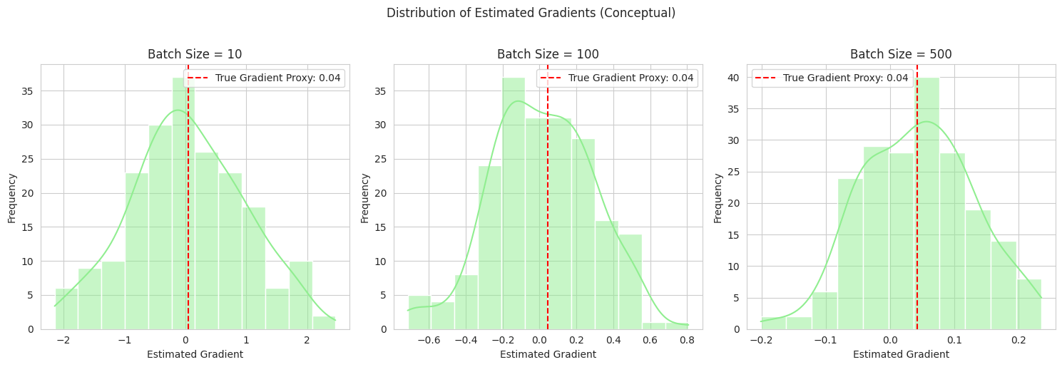
- We create a conceptual analogy to gradient estimation in machine learning. We have some "data," and we estimate a "gradient" (represented by the batch mean) using different batch sizes.
- We plot the distribution of these estimated gradients over multiple iterations for each batch size. This illustrates how using larger batches (taking a larger "sample" of the data to estimate the gradient) leads to a more stable and normally distributed estimate of the true gradient, which has implications for the training process of AI models.
Miscellenous
Try out: Colab Notebook