Linear Algebra
Based on the article “A Barebones Guide to Mechanistic Interpretability Prerequisites” written by Neel Nanda
Core goals - to deeply & intuitively understand these concepts:
Bonus things that it’s useful to understand:
1. Basis
To a 5-year old:
Imagine you have some LEGO blocks — a red block and a blue block.
With just those two types, you can build any shape on your LEGO board if you place enough of them in the right way.
The red and blue blocks are like your special building blocks — we call them a basis.
They are the blocks that help build everything else.
1
2
3
4
5
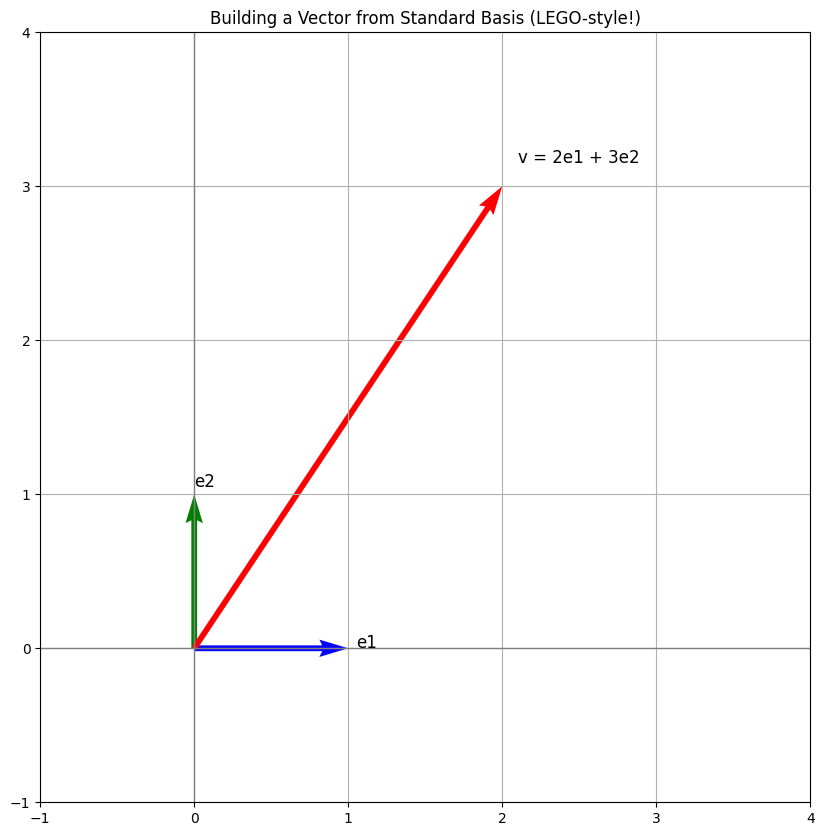
- The blue and green arrows show the **standard basis vectors**:
- e1=[1,0] → X-direction
- e2=[0,1] → Y-direction
- The **red arrow** shows a vector v=[2,3] in terms of these standard directions.
- This is how we usually think of vectors in 2D: how far right and how far up.
To a university student:
A basis in linear algebra is a set of vectors that are:
- Linearly independent — none of them can be written as a combination of the others.
- Span the space — any vector in that space can be written as a linear combination of these basis vectors.
For example, in 2D space, the vectors \(\mathbf{e}_1 = \begin{bmatrix} 1 \\ 0 \end{bmatrix}, \quad \mathbf{e}_2 = \begin{bmatrix} 0 \\ 1 \end{bmatrix}\)form the standard basis. Any 2D vector like \(\begin{bmatrix} 2 \\ 3 \end{bmatrix}\) can be made by:\(2 \cdot \mathbf{e}_1 + 3 \cdot \mathbf{e}_2\)You can choose other basis vectors too, as long as they follow the two rules.
1
2
3
4
5
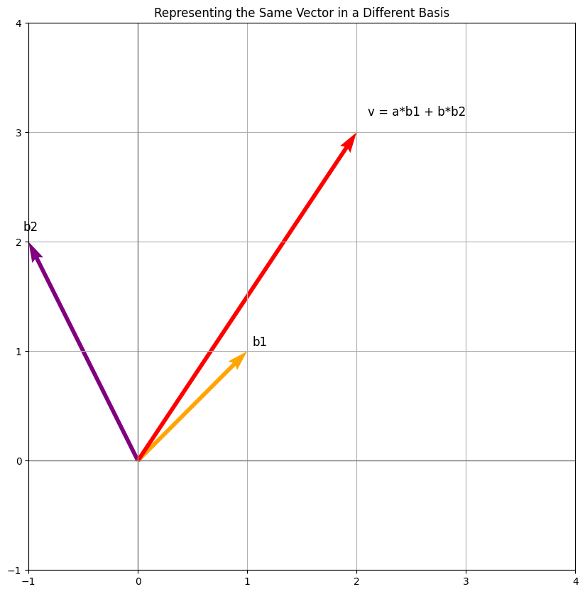
- The yellow and purple arrows represent the **new basis** vectors b1=[1,1] and b2=[0,2].
- The red arrow again shows the **same vector**, but now we're interpreting it using this new "ruler set" (basis).
- The vector’s coordinates are different in this new basis but still point to the same spot in space.
To an AI/ML Engineer:
A basis is a minimal set of vectors that represent a vector space. Any data point (vector) in that space can be expressed as a linear combination of these basis vectors.
Think of PCA (Principal Component Analysis): it finds a new basis aligned with the directions of maximum variance. The principal components become the new basis vectors, and data gets projected onto them to reduce dimensions or denoise.
In deep learning, basis concepts are implicit in:
- Representing embeddings in a lower-dimensional space.
- Understanding weight matrices (they transform inputs via basis change).
- Attention mechanisms linearly combining value vectors using learned attention weights.
A well-chosen basis reduces redundancy and allows more efficient representation and manipulation of data.
2. Change of Basis
To a 5-year old
Imagine you have a box of LEGOs. You can build things using red, blue, and yellow blocks. Let’s say these are your “first set” of building blocks.
Now, your friend has the same LEGOs, but they like to build using long, flat blocks and small, round blocks instead. These are their “second set” of building blocks.
Even though you’re using different kinds of blocks, you can still build the same castle! You just need to figure out how many of your blocks it takes to make one of your friend’s blocks, and vice versa.
“Change of basis” is like saying, “If my castle uses 2 red and 3 blue blocks, how many long and round blocks would my friend need to build the exact same castle?” We’re just looking at the same thing (the castle) using different sets of basic building blocks.
1
2
3
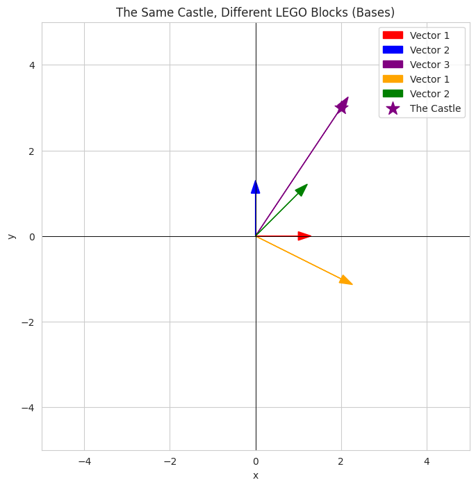
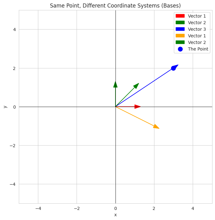
- We define two "sets" of basis vectors (`basis1` - red/blue, `basis2` - orange/green).
- The "castle" is a vector represented by coordinates in the first basis.
- The visualization shows the standard basis vectors, the new basis vectors, and the "castle" vector. The key is to see that the castle (purple star) is in the same location regardless of the underlying basis used to describe how to reach it. The code conceptually shows that a different combination of the friend's blocks would build the same castle.
To a university student
Think about describing the location of a point on a graph. Usually, we use the standard x and y axes. These axes define our “standard basis” vectors: \(\begin{bmatrix} 1 \\ 0 \end{bmatrix}\) (one step along \(x\)) and \(\begin{bmatrix} 0 \\ 1 \end{bmatrix}\) (one step along \(y\)). Any point \((x,y)\) can be seen as \(x\) times the \(x\)-basis vector plus \(y\) times the \(y\)-basis vector.
The same point in space hasn’t moved, but its coordinates (the numbers we use to describe its location) will be different because we’re using a different “ruler” (our new basis vectors) to measure its position.
“Change of basis” is the process of finding the new coordinates of a vector when we switch from one basis to another. It involves finding the relationship between the old basis vectors and the new basis vectors. This relationship is often represented by a change of basis matrix. Multiplying the original coordinate vector by this matrix gives you the new coordinate vector in the new basis.
1
2
3
4
5
-   We define the standard basis and a vector in that basis.
-   We define a new, "tilted" basis.
-   The `P_new_to_standard` matrix represents how to go from the new basis to the standard basis.
-   The `P_standard_to_new` matrix (the inverse) represents how to find the coordinates of a vector in the new basis given its coordinates in the standard basis.
-   The visualization shows the standard basis vectors, the new basis vectors, and the same point (blue dot) represented by its vector. The coordinates of the point are different relative to each basis.
To an AI/ML Engineer
In machine learning and AI, how we represent our data (features, embeddings, etc.) is crucial. Different representations can highlight different aspects of the data and can significantly impact the performance of our models.
Think of a dataset as a collection of vectors in a high-dimensional space. The initial way we represent these vectors (e.g., pixel values for images, word counts for text) defines a certain basis.
However, this initial basis might not be the most informative or efficient. Techniques like Principal Component Analysis (PCA) or feature learning aim to find a new basis that better captures the underlying structure of the data, often by reducing dimensionality or decorrelating features. This new basis can lead to more effective learning.
“Change of basis” is fundamental here. We are transforming our data from one representation (one basis) to another, often to simplify the problem, extract more meaningful features, or improve computational efficiency. The transformation matrix we use in these techniques is essentially a change of basis matrix.
Furthermore, in areas like robotics or computer graphics, we might need to work with different coordinate frames (different bases) to represent the position and orientation of objects. Understanding how to transform vectors between these frames using change of basis is essential for tasks like sensor fusion or object manipulation.
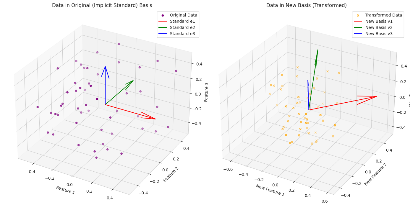
1
2
3
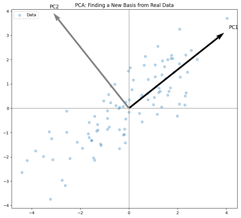
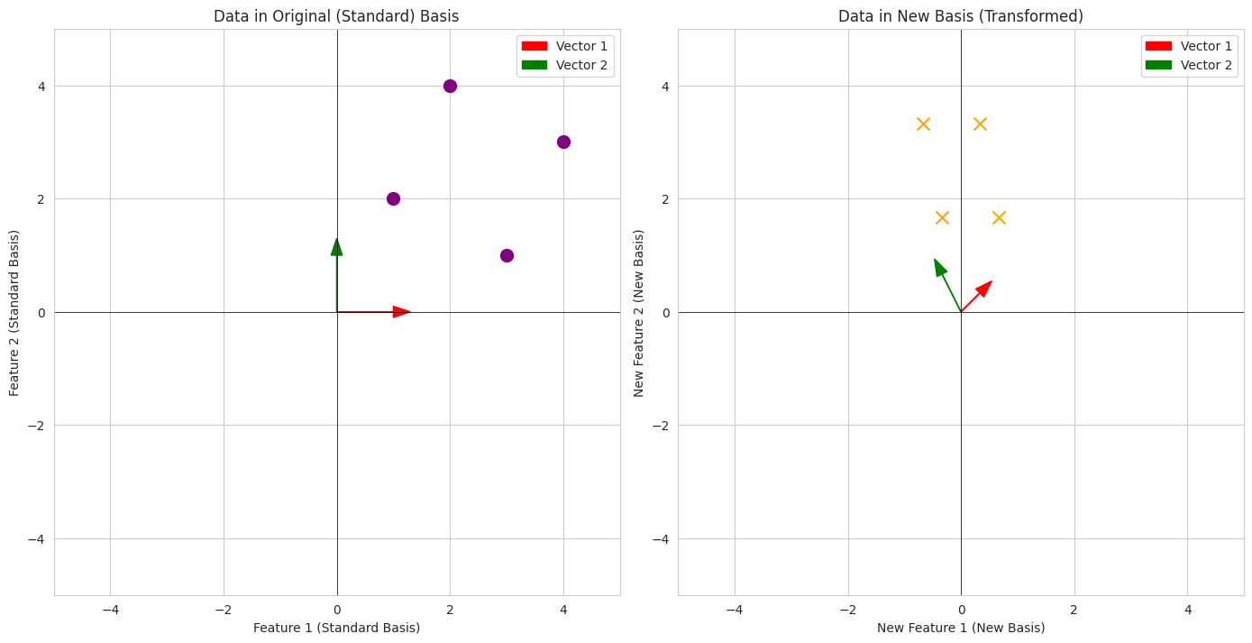
- We have sample data points, initially represented in an implicit "standard feature space."
- We use the same change of basis matrix as the undergrad student example to transform this data to a new representation (a new basis).
- The visualization shows the original data distribution relative to the standard axes and the transformed data distribution relative to the transformed axes. This illustrates how a change of basis can lead to a different way of looking at and representing the same data, which is crucial in feature engineering and dimensionality reduction.
3. A vector space is a geometric object that doesn’t necessarily have a canonical basis
To a 5-year old
Imagine you have a big empty playground (that’s our vector space!). You can put things on the playground, like a toy car. The car is at a certain spot.
Now, you want to tell your friend where the car is.
- You might say: “It’s 3 big steps forward and 2 small steps to the right from the swing!” (Your “big step” and “small step” are like your basis vectors).
- Your other friend might say: “It’s 4 sideways steps towards the slide and 1 long jump away from the tree!” (Their “sideways step” and “long jump” are their basis vectors).
The car is in the same spot on the playground, but you used different ways to describe how to get there. The playground itself didn’t tell you to use “big steps” and “small steps” or “sideways steps” and “long jumps.” You chose your own ways to explain it.
A vector space (the playground) is just the space where things can be. It doesn’t come with built-in directions or steps (a canonical basis). We pick our own directions (basis) to help us talk about where things are.
1
2
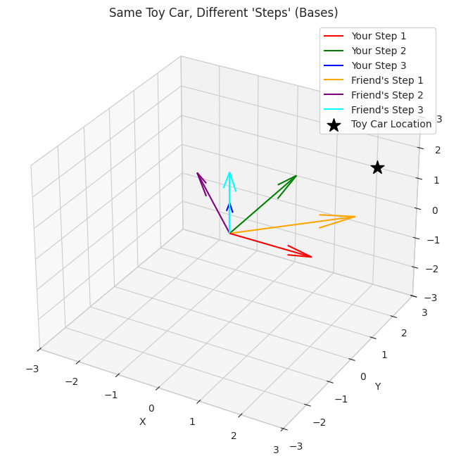
- We visualize a "toy car" at a specific location in 3D space.
- Two different sets of basis vectors (your "steps" and your friend's "steps") are plotted. The key takeaway is that the car's location is fixed, but it can be described using different sets of reference directions.
To a university student
Think of a vector space \(V\) as an abstract geometric entity – a set of objects (vectors) that can be added together and multiplied by scalars, satisfying certain axioms. This space exists independently of any specific coordinate system.
A basis for \(V\) is a set of linearly independent vectors that span \(V\). It provides a way to assign coordinates to every vector in \(V\). However, the choice of basis is not unique.
- Example in \(\mathbb{R^2}\): The standard basis \(\{\begin{bmatrix} 1 \\ 0 \end{bmatrix}, \quad \begin{bmatrix} 0 \\ 1 \end{bmatrix} \}\)is convenient. But \(\{\begin{bmatrix} 1 \\ 1 \end{bmatrix}, \quad \begin{bmatrix} -1 \\ 1 \end{bmatrix} \}\) is also a valid basis. The vector \(\begin{bmatrix} 3 \\ 2 \end{bmatrix}\) can be represented in both bases with different coordinates. The underlying vector (the geometric arrow) is the same.
The term “canonical basis” would imply a single, natural, or inherently preferred basis for the vector space itself. While some vector spaces have a commonly used or “standard” basis (like the standard basis for \(\mathbb{R^n}\)), this choice is often due to convenience or convention, not an intrinsic property of the vector space’s geometry.
The vector space as a geometric object (the plane, 3D space, the space of polynomials) doesn’t inherently dictate which set of “measuring sticks” (basis vectors) we must use. We choose a basis that is convenient for the problem at hand.
1
2
3
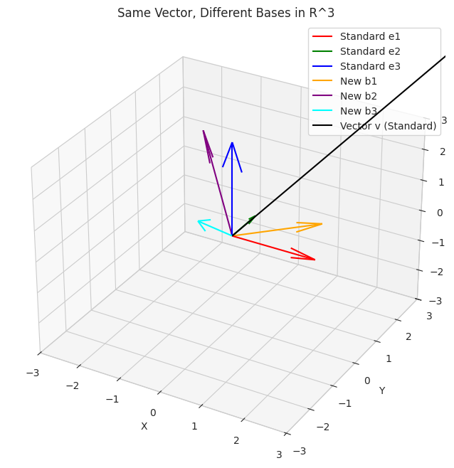
- We visualize the standard basis vectors for R^3 (red, green, blue arrows along the x, y, and z axes).
- We also plot another valid basis for R^3 (orange, purple, cyan arrows, which are linear combinations of the standard basis).
- A vector `v` is plotted. You can see that this same vector can be described using coordinates relative to the standard basis or relative to the new basis. The geometric arrow itself doesn't change.
To an AI/ML Engineer
In AI/ML, we work with data represented as vectors in high-dimensional spaces (feature spaces, embedding spaces). The initial way we represent this data defines a basis.
- Example in Image Processing: An image can be represented by its pixel values (a vector in a high-dimensional space where each dimension corresponds to a pixel). This is one basis. However, we could transform this representation using techniques like Fourier Transform or Wavelet Transform, which effectively change the basis to one that might highlight different features (frequencies, edges). The underlying image (the geometric object) remains the same, but its numerical representation changes with the basis.
The concept that a vector space doesn’t have a canonical basis is crucial because it highlights the flexibility of representation. We are not stuck with the initial, often arbitrary, way our data is presented. We can choose or learn new bases that are more suitable for our tasks (e.g., for better feature extraction, dimensionality reduction, or improved model performance).
Techniques like Principal Component Analysis (PCA) explicitly find a new basis (principal components) that captures the directions of maximum variance in the data. This new basis is often more informative than the original feature basis. Similarly, learned representations in neural networks can be seen as transformations to new, data-driven bases.
The lack of a canonical basis empowers us to engineer features and learn representations that are tailored to the specific problem and data, rather than being constrained by an arbitrary initial representation.
1
2
3
4
-   We generate some random 3D data points. Initially, these are implicitly represented using the standard basis (each feature corresponds to one standard basis direction).
-   We define an arbitrary `transformation_matrix` and use its transpose as a new basis. In a real AI/ML scenario, this matrix might be learned or computed (e.g., from PCA).
-   We transform the original data to the new basis.
-   The visualization shows the original data distribution and the transformed data distribution. The change of basis rotates and potentially scales the data, leading to a different representation that might be more useful for subsequent analysis or modeling. The new basis vectors are also plotted to show the new coordinate system.
4. A matrix is a linear map between two vector spaces (or from a vector space to itself)
To a 5-year old:
Imagine you’re putting stickers on paper.
- You have a special machine (the matrix) that tells you where to put the stickers.
- If you give it one spot (a vector), the machine will move it to another spot.
- The machine always moves them in a straight and predictable way.
- So the matrix is like a magic rule that moves your stickers from one place to another — always in the same kind of way.
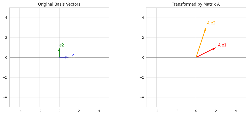
To a university student
A matrix is more than a grid of numbers — it represents a function (or transformation) that takes input vectors from one vector space and outputs new vectors in another space, while preserving two important properties:
- Additivity: \(M(v + w) = Mv + Mw\)
- Homogeneity: \(M(c·v) = c·(Mv)\)
This makes it a linear map.
For example:
- A \(3×2\) matrix maps 2D vectors → 3D space.
- A \(2×2\) matrix rotates or scales vectors within the 2D plane.
The matrix gives us a structured way to compute how vectors move between or within spaces.
To a AI/ML engineer
In practical terms:
A matrix \(A\) is a linear transformation \(A: V → W\), where:
- \(V\) and \(W\) are vector spaces (often \(\mathbb{R^n}\) and \(\mathbb{R^m}\)),
- The matrix applies a consistent, linear rule to transform vectors.
This is fundamental in ML:
- Weight matrices in neural nets are linear maps that transform activations across layers.
- PCA uses a change of basis to map data to a space of principal components — again, done via a matrix.
- In attention mechanisms, the \(Q\), \(K\), and \(V\) projections are learned matrices mapping inputs to new spaces.
In summary: Matrices are compact representations of linear operators that drive most of the transformations in modern AI models.
5. What’s singular value decomposition? Why is it useful?
To a 5-year old
Imagine you have a bunch of pictures of different things – cats, dogs, trees, houses.
What’s SVD? It’s like a special way to:
- Find the most important “shapes” or “patterns” in all your pictures. Maybe most cat pictures have pointy ears, and most dog pictures have floppy ears. These pointy and floppy ears are like the most “singular” or special features.
- Sort the pictures based on how much of these important shapes they have. Pictures with very pointy ears go in one group, pictures with very floppy ears go in another.
- Make a simpler version of each picture by only keeping the most important shapes. If pointy ears are the most important thing for cats, we can make a simpler cat picture that mostly shows the pointy ears.
Why is it useful?
- Sorting: It helps you sort your pictures in a smart way based on what’s most important.
- Simplifying: It lets you make smaller, easier-to-see versions of your pictures by getting rid of less important details, but still keeping the main idea. This is like making a quick sketch of a cat that mostly shows its pointy ears so you know it’s a cat.
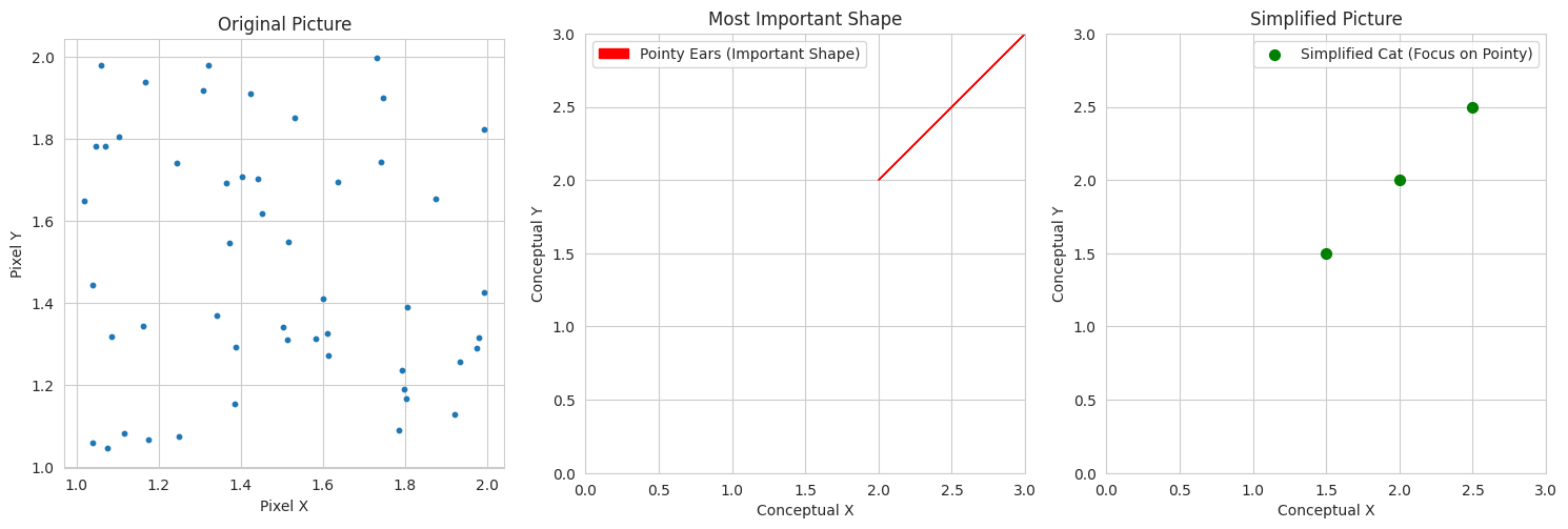
1
2
3
-   We create a conceptual visualization. The original "complex" cat picture is represented by many points.
-   The "most important shape" (pointy ears) is shown as an arrow representing a dominant feature.
-   The "simplified" picture focuses on this important shape with fewer details. This conceptually shows how SVD helps focus on the most significant aspects.
To a university student
Singular Value Decomposition (SVD) is a powerful matrix factorization technique. For any real or complex matrix \(M\) of size \(m×n\), SVD decomposes it into the product of three other matrices:
\[M=UΣV^T\]Where:
- \(U\) is an \(m×m\) unitary matrix (its columns are orthonormal eigenvectors of \(MM^T\)). The columns of \(U\) are called the left-singular vectors of \(M\).
- \(Σ\) is an \(m×n\) rectangular diagonal matrix with non-negative real numbers on the diagonal, called the singular values of \(M\). These singular values are usually arranged in descending order.
- \(V^T\) is the transpose of an \(n×n\) unitary matrix (its rows are orthonormal eigenvectors of \(M^TM\)). The columns of \(V\) (so the rows of \(V^T\)) are called the right-singular vectors of \(M\).
Why is it useful?
- Dimensionality Reduction: The singular values in \(Σ\) represent the “strength” or importance of the corresponding singular vectors in \(U\) and \(V\). By keeping only the largest \(k\) singular values and their corresponding singular vectors, we can obtain a low-rank approximation of the original matrix \(M_k=U_kΣ_kV_k^T\) that captures most of the variance or information in the data. This is crucial for reducing the dimensionality of high-dimensional datasets while preserving essential information.
- Data Compression: Similar to dimensionality reduction, by using a low-rank approximation, we can represent the original matrix with fewer numbers, leading to data compression.
- Noise Reduction: Smaller singular values often correspond to noise or less significant variations in the data. By discarding these, the low-rank approximation can effectively denoise the data.
- Latent Semantic Analysis (LSA): In natural language processing, SVD can be used to uncover underlying semantic relationships between documents and terms. The singular vectors can represent abstract topics, and the singular values indicate their importance.
- Recommender Systems: SVD can be applied to user-item interaction matrices to discover latent factors representing user preferences and item characteristics, enabling personalized recommendations.
- Solving Linear Systems: SVD can be used to find the pseudoinverse of a matrix, which is helpful in solving overdetermined or underdetermined linear systems, especially when the matrix is singular or ill-conditioned.
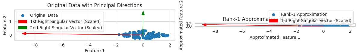
1
2
3
4
-   We generate 2D data that is stretched along a principal direction.
-   We perform SVD on this data.
-   We plot the original data and the first and second right-singular vectors (scaled by singular values), which represent the principal directions.
-   We then show a rank-1 approximation of the data, which is the best 1-dimensional representation of the data in the direction of the first singular vector. This illustrates dimensionality reduction.
To a AI/ML engineer
Singular Value Decomposition (SVD) is a fundamental linear algebra technique that provides a powerful way to decompose a data matrix into a product of three matrices that reveal the principal components or latent factors within the data. Given a data matrix \(X∈\mathbb{R}^{m×n}\) (where \(m\) is the number of samples and \(n\) is the number of features), SVD gives:
\[X=UΣV^T\]Where:
- \(U∈\mathbb{R}^{m×m}\) contains the left-singular vectors, representing the principal directions in the sample space.
- \(Σ∈ \mathbb{R}^{m×n}\) is a diagonal matrix with singular values \(σ1≥σ2≥⋯≥0\) on the diagonal, indicating the importance or variance captured by the corresponding singular vectors.
- \(V∈\mathbb{R}^{n×n}\) contains the right-singular vectors, representing the principal directions in the feature space.
Why is it useful?
- Principal Component Analysis (PCA): SVD is the core mathematical engine behind PCA, a widely used dimensionality reduction technique. By taking the top k singular vectors in V (corresponding to the k largest singular values), we can project the data onto a lower-dimensional subspace that captures the most variance.
- Recommendation Systems (Matrix Factorization): In collaborative filtering, SVD-like techniques are used to factorize the user-item interaction matrix into lower-dimensional user and item latent factor matrices. This allows for predicting missing ratings and generating recommendations.
- Natural Language Processing (NLP):
- Latent Semantic Analysis (LSA) / Latent Semantic Indexing (LSI): SVD can uncover hidden semantic relationships between documents and terms in a document-term matrix.
- Word Embeddings: While more modern techniques like Word2Vec and GloVe are prevalent, the underlying idea of dimensionality reduction to capture semantic meaning is related to the principles of SVD.
- Image Compression: By performing SVD on an image matrix and keeping only the top singular values and vectors, we can achieve significant image compression while retaining the most important visual information.
- Noise Reduction: By discarding singular values below a certain threshold, we can filter out noise and retain the underlying signal in the data.
- Understanding Data Variance: The singular values provide a direct measure of the variance captured along the principal components. This helps in understanding the intrinsic dimensionality and structure of the data.
- Initialization Techniques: In some deep learning models, SVD can be used for weight initialization to provide a more structured starting point for training.
1
2
3
4
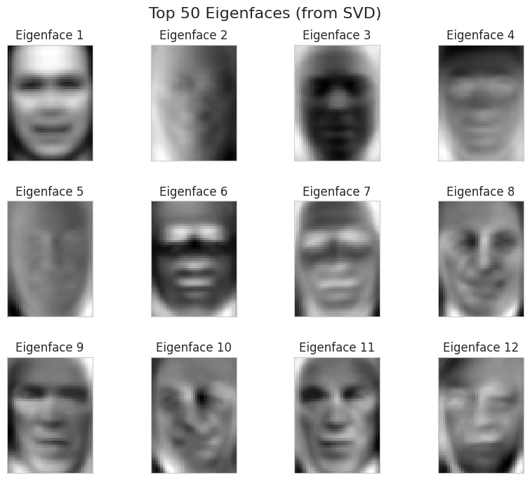
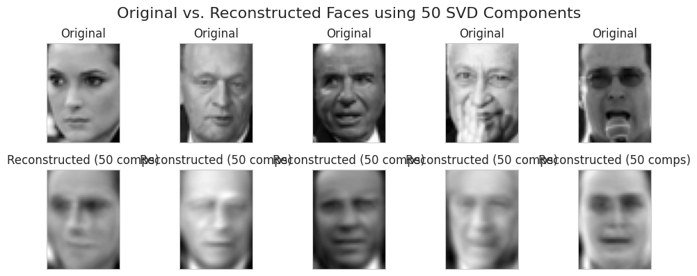
- We use the "LFW Faces" dataset, a common dataset in computer vision.
- We apply `TruncatedSVD` (an efficient version of SVD for large, sparse matrices, often used in PCA).
- We visualize the top `n_components` "eigenfaces" (which are related to the right-singular vectors and represent the principal components of the face data). These are the most important patterns in the faces.
- We then show a few original faces and their reconstructions using only these `n_components`. You can see that even with a much lower dimensionality, the reconstructed faces still retain the main characteristics. This demonstrates the power of SVD for dimensionality reduction and feature extraction in AI/ML.
6. Orthogonal and orthonormal matrices and the importance of changing to an orthonormal basis
To a 5-year old:
Imagine you’re building with LEGOs again.
- Orthogonal: Think of blocks that fit together perfectly at right angles (like regular square or rectangular blocks). They stand straight up and down or side by side, making nice, neat corners. They don’t lean on each other in a funny way.
- Orthonormal: Now, imagine those perfectly square blocks are also all exactly the same size (say, 1x1 squares). They fit together perfectly at right angles AND they are all the same “unit” size.
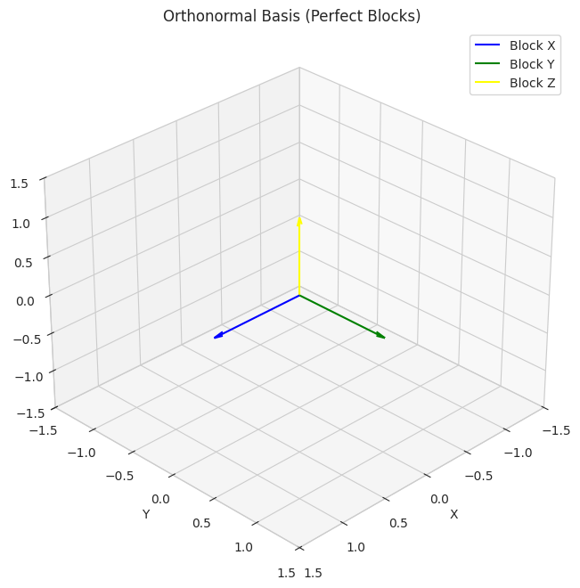
- Changing to an orthonormal basis (using only these perfect square blocks of the same size): It’s like building your LEGO castle using only these nice, regular blocks. Everything stays the right shape and size. If your castle is 5 blocks long in one direction, it will still be 5 “units” long even if you turn your castle around. The distances and angles inside your castle stay the same.
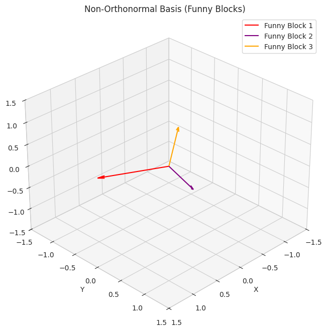
- Changing to just any basis (using funny-shaped or different-sized blocks): Imagine if your friend built their castle using long, slanted blocks and tiny round blocks. The shape of their castle might look the same overall, but the lengths and angles inside would be all stretched and weird compared to yours. Measuring things in their castle would be much harder because their “blocks” aren’t regular.
Why is using the perfect square blocks (orthonormal basis) important? It keeps everything nice and easy to measure. The real shape and size of things don’t get distorted just because you’re looking at them from a different angle or using a different set of building blocks.
1
2
-   We show two sets of basis vectors in 3D. The first set (`orthonormal_basis`) is aligned with the axes and represents "perfect square blocks."
-   The second set (`non_orthonormal_basis`) is skewed, representing "funny-shaped blocks." The visualization helps understand that using the perfect blocks keeps things regular and easier to understand geometrically.
To a university student:
Orthogonal Matrices:
- A real square matrix \(Q\) is orthogonal if its transpose is equal to its inverse: \(Q^T=Q^{−1}\)
- This implies that \(Q^TQ=I\) and \(QQ^T=I\), where \(I\) is the identity matrix.
- Geometrically, the columns (and rows) of an orthogonal matrix are orthogonal vectors (their dot product is zero) and have a magnitude (norm) of 1 (they are unit vectors). Such a set of vectors is called an orthonormal set.
- An orthogonal matrix represents a linear transformation that preserves lengths (norms) and angles between vectors. These transformations include rotations, reflections, and permutations.
Orthonormal Matrices:
- For real matrices, an orthonormal matrix is the same as an orthogonal matrix as defined above. The term “orthonormal” emphasizes that the columns (and rows) form an orthonormal set.
Why is changing to an orthonormal basis importantly different from just any change of basis?
Preservation of Geometric Properties:
- Lengths: When you represent a vector in an orthonormal basis, its Euclidean norm (length) is preserved under the change of basis. If \(v\) has coordinates \([v]_B\) in an orthonormal basis \(B\) and \([v]_C\) in another orthonormal basis \(C\), then \(∣∣v∣∣_2=∣∣[v]_{B∣∣2}=∣∣[v]_{C∣∣2}\). This is not generally true for a non-orthonormal change of basis.
- Angles: The angles between vectors are also preserved when changing between orthonormal bases. The dot product between two vectors is directly related to the cosine of the angle between them, and the dot product is preserved (up to a sign if a reflection is involved).
- Distances: Since lengths are preserved, the distances between points (represented by vectors) are also preserved.
Simplified Calculations:
- Inverse: The inverse of an orthogonal matrix is simply its transpose, which is computationally much cheaper to compute than the general inverse. This simplifies many linear algebra operations.
- Projections: Orthogonal projections onto subspaces spanned by orthonormal bases have simpler formulas.
- Coordinate Transformation: The change of basis matrix between two orthonormal bases is itself an orthogonal matrix.
Numerical Stability: Computations involving orthonormal bases and orthogonal matrices tend to be more numerically stable, reducing the accumulation of rounding errors in computer calculations.
Physical Interpretations: In physics and engineering, many natural coordinate systems are orthonormal (e.g., Cartesian coordinates). Transformations between these systems often involve orthogonal matrices, reflecting the preservation of physical quantities like length and energy.
1
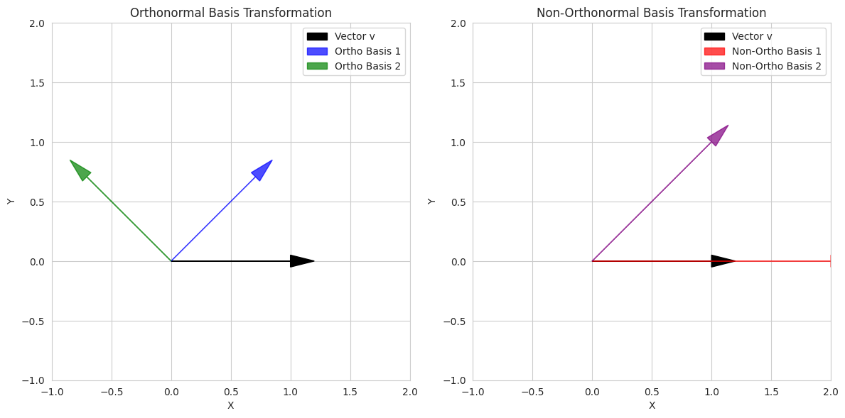
2
3
- We demonstrate the effect of changing to an orthonormal basis (a rotation matrix `Q`) and a non-orthonormal basis (`A`) on a vector `v`.
- We print the magnitudes of the vector in both bases. You'll see that the magnitude is preserved under the orthonormal transformation but not the non-orthonormal one.
- The plots show the original vector and the basis vectors for both transformations, visually illustrating how the non-orthonormal basis can stretch or skew the space.
To a AI/ML Engineer
Orthogonal/Orthonormal Matrices:
- Orthogonal (for real-valued data) or unitary (for complex-valued data) matrices are square matrices whose columns (and rows) form an orthonormal set of vectors.
- \(Q^TQ=I\) (for real orthogonal matrices).
- \(Q^HQ=I\) (for complex unitary matrices, where \(Q^H\) is the conjugate transpose).
Why is changing to an orthonormal basis importantly different from just any change of basis?
- Preserving Data Geometry:
- When transforming data to an orthonormal basis, the Euclidean distances between data points and the angles between feature vectors are preserved. This is crucial in many ML algorithms where these geometric relationships are important (e.g., nearest neighbors, clustering, kernel methods).
- Transformations to non-orthonormal bases can distort these relationships, potentially affecting the performance of geometric algorithms.
- Simplified Computations and Inverses:
- The ease of inverting orthogonal matrices \((Q^{−1}=Q^T)\) is highly beneficial computationally, especially in high-dimensional spaces. This is used in various algorithms, including some forms of whitening and decorrelation.
Decorrelation of Features: Transforming data to a basis where the basis vectors are orthogonal often leads to decorrelated features. This can be advantageous for some models (e.g., simplifying covariance matrices in Gaussian models, improving the efficiency of optimization algorithms). PCA, which relies on finding an orthonormal basis of principal components, is a prime example.
Numerical Stability in Algorithms: Many numerical algorithms used in AI/ML (e.g., optimization routines, eigenvalue solvers) benefit from working with orthonormal bases and orthogonal matrices, as they tend to be more numerically stable and less prone to error propagation.
Initialization of Neural Networks: Orthogonal initialization schemes for neural network weight matrices are often used to improve training stability and prevent issues like vanishing or exploding gradients. By starting with orthogonal weights, the variance of the signals propagated through the network is better controlled.
- Rotations and Reflections as Building Blocks: Orthogonal matrices represent fundamental geometric transformations like rotations and reflections, which are essential components in many AI/ML models and data processing pipelines (e.g., image augmentation, geometric transformations in computer vision).
1
2
3
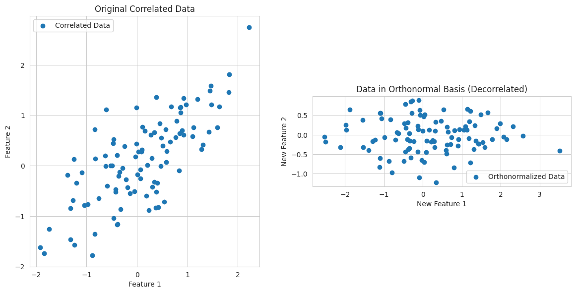
- We generate correlated 2D data.
- We conceptually perform an orthonormalizing transformation using the eigenvectors from SVD (similar to what PCA does). This rotates the data to a new basis where the features are uncorrelated (orthogonal).
- The plots show the original correlated data and the transformed, decorrelated data in the new orthonormal basis. This highlights the importance of orthonormal bases for simplifying data structure and improving model performance in some cases.
7. What are eigenvalues and eigenvectors, and what do these tell you about a linear map?
To a 5-year old
Imagine you have a magical arrow. When a special wind blows (that’s like a linear map or a matrix), the arrow usually changes direction and gets longer or shorter.
Now, sometimes, when this special wind blows on your magical arrow, something really cool happens:
- The arrow stays pointing in the exact same direction (or exactly opposite direction). It doesn’t turn at all!
- It might get longer or shorter, but it’s still on the same line.
The special direction that the arrow doesn’t change is called the eigenvector of the wind (the linear map).
How much longer or shorter the arrow gets is called the eigenvalue of that direction. If the eigenvalue is bigger than 1, the arrow gets longer. If it’s between 0 and 1, it gets shorter. If it’s negative, it flips to the opposite direction.
So, eigenvalues and eigenvectors tell you about the special directions where the “wind” only stretches or shrinks things, without changing their direction.
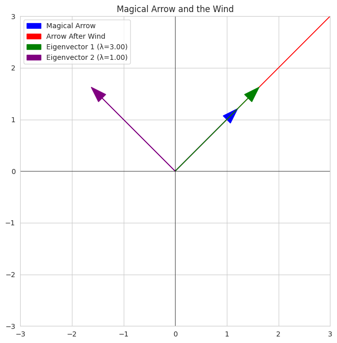
1
2
3
-   We define a "wind" (a 2x2 matrix) that transforms arrows.
-   We show a "magical arrow" and how it changes after the wind.
-   We then plot the eigenvectors of the "wind." Notice how these eigenvectors point in directions that the transformed arrow seems to be aligned with (just stretched). The eigenvalues tell us how much stretching occurs along these special directions.
To a university student
Consider a linear map \(T:V→V\) from a vector space \(V\) to itself (represented by a square matrix \(A\) when a basis is chosen).
An eigenvector \(v\) of \(T (or A)\) is a non-zero vector in \(V\) such that when \(T\) is applied to \(v\), the result is a scalar multiple of \(v\):
\[T(v)=λv\]where \(λ\) is a scalar called the eigenvalue associated with the eigenvector \(v\).
What do these tell you about a linear map?
Invariant Directions/Subspaces: Eigenvectors represent directions in the vector space that are invariant under the linear transformation \(T\), meaning that the transformation only scales the vector along its original direction; it doesn’t rotate or move it off the line spanned by \(v\). The subspace spanned by an eigenvector is an invariant subspace of \(T\).
Scaling Factors: The eigenvalue \(λ\) tells you the factor by which the eigenvector is scaled by the transformation.
- \(∣λ∣>1\): Stretching along the eigenvector’s direction.
- \(0<∣λ∣<1\): Shrinking along the eigenvector’s direction.
- \(λ=1\): The eigenvector remains unchanged.
- \(λ=−1\): The eigenvector is flipped to the opposite direction with the same magnitude.
- \(λ=0\): The eigenvector is mapped to the zero vector (it lies in the null space of \(T\)).
Diagonalization: If a matrix \(A\) has a full set of linearly independent eigenvectors, it can be diagonalized. This means we can find an invertible matrix \(P\) whose columns are the eigenvectors of \(A\), and a diagonal matrix \(D\) whose diagonal entries are the corresponding eigenvalues, such that: \(A=PDP^{−1}\)
This diagonalization simplifies many matrix operations, such as computing powers of a matrix \((A_k=PD_kP^{−1})\) and solving systems of linear differential equations.
Understanding the Action of the Linear Map: Eigenvalues and eigenvectors provide a fundamental understanding of how a linear map acts on the vector space. They reveal the “principal axes” or the most important directions of transformation. By analyzing the eigenvalues and eigenvectors, we can decompose the linear transformation into simpler scaling operations along these special directions.
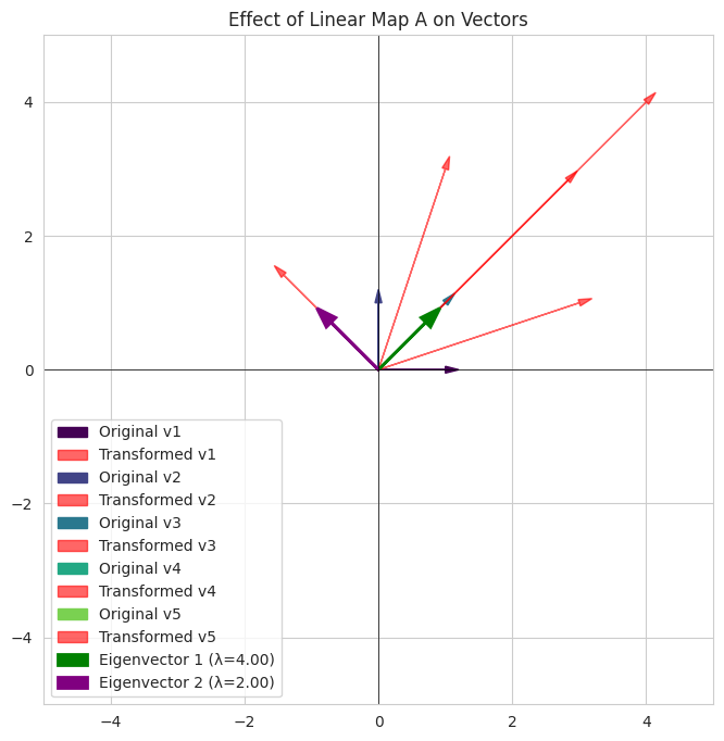
1
2
3
-   We define a 2x2 matrix `A` representing a linear map.
-   We find its eigenvalues and eigenvectors.
-   We visualize how `A` transforms several original vectors. Observe that the eigenvectors (green and purple arrows) are only stretched or shrunk by the transformation (red arrows originating from them), staying along the same line. Other vectors change direction.
To a AI/ML Engineer
What are eigenvalues and eigenvectors?
For a square matrix \(A\) representing a linear transformation in a feature space, eigenvectors \(v\) are the directions that remain unchanged (or just flipped) by the transformation, and eigenvalues \(λ\) are the scaling factors associated with these directions:
\[Av=λv\]What do these tell you about a linear map (and data)?
Principal Components (PCA): In Principal Component Analysis, we compute the eigenvalues and eigenvectors of the covariance matrix of the data. The eigenvectors with the largest eigenvalues correspond to the principal components – the directions of maximum variance in the data. The eigenvalues indicate the amount of variance captured along each principal component, signifying the importance of each direction.
Feature Importance: In some contexts, eigenvalues can indicate the “strength” or importance of certain features or directions in the data space after a linear transformation. Larger eigenvalues often correspond to more significant axes of variation.
Stability Analysis: In dynamical systems and recurrent neural networks, eigenvalues of the weight matrices can determine the stability of the system. Eigenvalues with magnitudes less than 1 indicate stability, while magnitudes greater than or equal to 1 suggest instability (e.g., exploding gradients).
Spectral Analysis: The spectrum of a matrix (the set of its eigenvalues) provides insights into the properties of the linear transformation it represents. For example, the magnitude of the largest eigenvalue (spectral radius) is related to the convergence rate of iterative algorithms.
Graph Analysis: Eigenvalues and eigenvectors of graph adjacency matrices (or related matrices like the Laplacian) are used in spectral graph theory for tasks like community detection, graph partitioning, and ranking nodes. The eigenvectors can reveal important structural properties of the graph.
Recommendation Systems (Matrix Factorization): In some matrix factorization techniques like SVD (which is related to eigenvalue decomposition for symmetric matrices), singular values (square roots of eigenvalues of ATA or AAT) indicate the importance of latent factors. The singular vectors (related to eigenvectors) represent the directions of these factors in the user and item spaces.
Image Compression: Eigenvalue decomposition-like techniques (e.g., in Karhunen-Loève transform, which is equivalent to PCA) can be used for image compression by keeping only the eigenvectors corresponding to the largest eigenvalues, which capture the most important visual information.
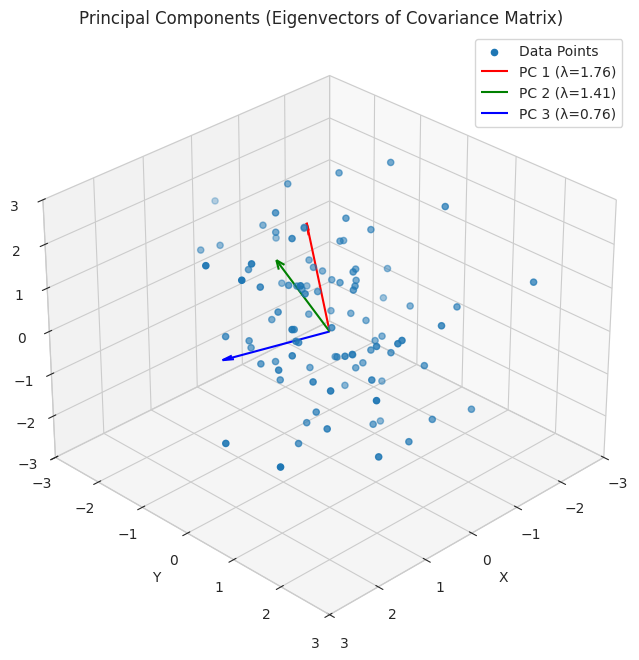
1
2
3
-   We simulate 3D data with some correlation between the features.
-   We compute the covariance matrix of the data, which describes the relationships between the features.
-   We find the eigenvalues and eigenvectors of the covariance matrix. The eigenvectors (plotted as red, green, and blue arrows, scaled by the square root of the eigenvalues) represent the principal components – the directions of maximum variance in the data. The eigenvalues indicate the amount of variance along each principal component, showing the importance of each feature direction.
Miscellenous
Try out: Colab Notebook