Calculus Basics
Based on the article “A Barebones Guide to Mechanistic Interpretability Prerequisites” written by Neel Nanda
Gradients
To a 5-year old
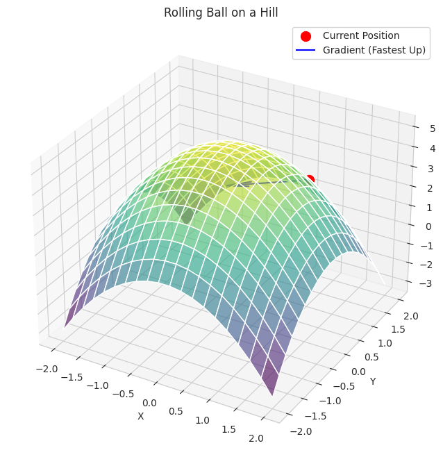
Imagine you’re rolling a ball on a bumpy hill.
The Hill: The hill goes up and down in different directions.
Gradient (The Fastest Way Up): If you’re standing at one spot on the hill and you want to get to the very top as quickly as possible, the “gradient” is like the arrow that points in the direction of the steepest uphill climb right from where you are. It also tells you how steep that climb is.
Big Arrow: If the hill is very steep in one direction, the gradient arrow will be long.
Gentle Slope: If the hill is only gently sloping, the arrow will be short.
So, the gradient always points you to the fastest way to go up the hill from your current spot!
1
2
3
-   We define a simple "hill" function in 3D.
-   We plot the hill and a red ball at a starting position.
-   A blue arrow (the gradient) shows the direction of the steepest upward climb from the ball's location.
To an undergraduate student
In multivariable calculus, the gradient of a scalar function $f(x_1,x_2,…,x_n)$ is a vector field denoted by $∇f$ (nabla $f$) or grad $f$. It points in the direction of the greatest rate of increase of the function at a given point, and its magnitude is the rate of increase in that direction.
For a function $f(x,y)$ of two variables, the gradient is:
\[∇f(x,y)=(∂x/∂f,∂y/∂f)=\frac{∂x}{∂f}i+\frac{∂y}{∂f}j\]For a function $f(x,y,z)$ of three variables, the gradient is:
\[∇f(x,y,z)=(∂x/∂f,∂y/∂f,∂z/∂f)=\frac{∂x}{∂f}i+\frac{∂y}{∂f}j+\frac{∂z}{∂f}k\]In general, for $f(x_1,…,x_n)$, the gradient is:
\[∇f(x_1,...,x_n)=(\frac{∂x_1}{∂f},\frac{∂x_2}{∂f},...,\frac{∂x_n}{∂f})\]Key Properties of the Gradient:
- Direction of Steepest Ascent: $∇f(a)$ at a point a points in the direction in which $f$ increases most rapidly.
- Magnitude of Steepest Ascent: The magnitude $∣∣∇f(a)∣∣$ is the rate of increase of $f$ in that steepest direction.
- Relationship to Level Curves/Surfaces: The gradient at a point is always perpendicular (orthogonal) to the level curve (in 2D) or level surface (in 3D) passing through that point.
- Directional Derivative: The directional derivative of $f$ at $a$ in the direction of a unit vector $u$ is given by $D_uf(a)=∇f(a)⋅u$. This shows how the gradient can be used to find the rate of change of the function in any direction.
1
2
3
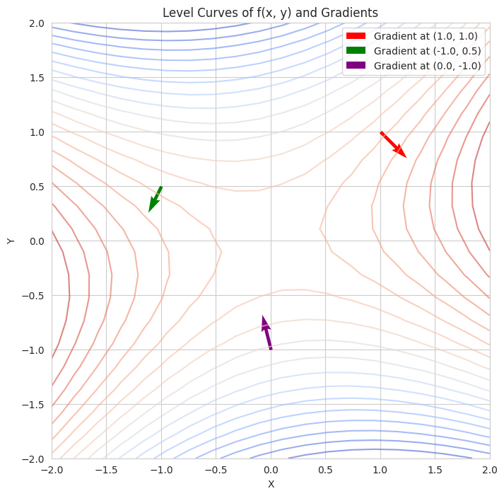
- We define a multivariable function `f(x, y)` and its gradient.
- We plot the level curves of the function (lines where the function has a constant value).
- At a few different starting points, we plot the gradient vectors. Notice how these vectors are perpendicular to the level curves at those points and indicate the direction of the steepest increase.
To an AI/ML engineer
In AI/ML, the concept of the gradient is absolutely fundamental, especially in the context of training machine learning models using optimization algorithms.
Loss Functions: Machine learning models are typically trained by minimizing a loss function $J(θ)$ with respect to the model’s parameters $θ$ (which can be weights and biases). The loss function quantifies the error between the model’s predictions and the true values.
Gradient Descent: The most common optimization algorithm used to minimize the loss function is gradient descent. The core idea is to iteratively update the parameters $θ$ in the direction opposite to the gradient of the loss function with respect to those parameters:
\(θ_{new}=θ_{old}−α∇_J(θ_{old})\) where $α$ is the learning rate, a positive scalar that determines the step size in the direction of the negative gradient.
Why the Negative Gradient? Since the gradient points in the direction of the steepest increase of the function, the negative gradient $−∇J(θ)$ points in the direction of the steepest decrease. By moving in this direction, we aim to find the parameter values that minimize the loss.
Backpropagation: In training neural networks, the backpropagation algorithm is an efficient way to compute the gradient of the loss function with respect to all the weights in the network. It uses the chain rule of calculus to propagate the error backwards through the network layers.
Optimization Algorithms: Many advanced optimization algorithms used in deep learning (e.g., Adam, SGD with momentum, RMSprop) are based on the concept of the gradient but incorporate various techniques to improve convergence speed and stability. These algorithms often adapt the learning rate or use information from past gradients.
Understanding Model Behavior: The gradient can also provide insights into the sensitivity of the model’s output with respect to changes in its input features or parameters.
1
2
3
4
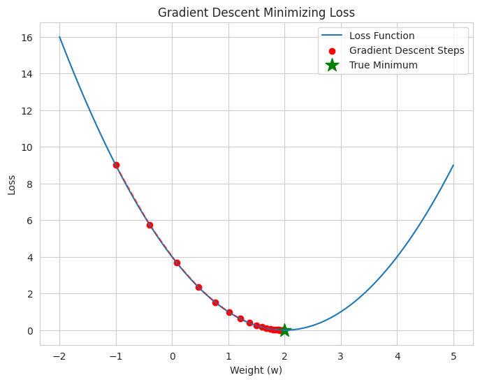
- We define a simple quadratic "loss function" (representing the error of a model with a single weight).
- We also define the gradient of this loss function with respect to the weight.
- We simulate gradient descent: starting with an initial weight, we iteratively update the weight by moving in the opposite direction of the gradient.
- The plot shows the loss function and the steps taken by gradient descent, illustrating how it moves towards the minimum of the loss.
The Chain rule
To a 5-year old
Imagine you’re building a really tall tower with LEGOs. You have small blocks that you put together to make bigger blocks, and then you stack the bigger blocks to make the tower.
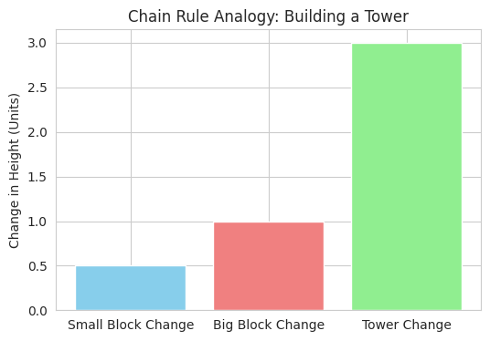
Changing the Big Blocks: If you add one more small block to each of your big blocks, how much taller does each big block get?
Changing the Whole Tower: Now, because each big block got a little taller, the whole tower also gets taller.
The chain rule is like saying: How much the whole tower changes depends on how much each big block changes, AND how many big blocks you have stacked up.
If the small blocks make the big blocks much taller, and you have many big blocks, the whole tower will get much, much taller!
1
We use a bar chart to illustrate the step-by-step change in height when building a tower. The change in small blocks leads to a change in big blocks, which in turn leads to a change in the total tower height, analogous to the chain rule linking rates of change.
To an undergraduate student
The chain rule is a fundamental rule in calculus that allows you to find the derivative of a composite function. If we have a function $y=f(u)$ and $u=g(x)$, then $y$ is a composite function of $x, y=f(g(x))$. The chain rule states that the derivative of $y$ with respect to $x$ is given by:
\[\frac{dy}{dx}=\frac{dy}{du}⋅\frac{du}{dx}\]In Leibniz notation, this shows that the rate of change of $y$ with respect to $x$ is the product of the rate of change of $y$ with respect to the intermediate variable $u$, and the rate of change of $u$ with respect to $x$.
Alternatively, using prime notation:
\[(f(g(x)))^′=f^′(g(x))⋅g^′(x)\]This means you take the derivative of the outer function $f$ with respect to its argument $g(x)$, and then multiply by the derivative of the inner function $g$ with respect to $x$.
Generalization to Multivariable Calculus:
For a function $f(x_1(t),x_2(t),…,x_n(t))$ where each $x_i$ is a function of $t$, the chain rule becomes:
\(\frac{df}{dt}=\frac{∂f}{∂x1} \frac{dx_1}{dt} +\frac{∂f}{∂x_2} \frac{dx_2}{dt}+...+\frac{∂f}{∂x}\frac{dx_n}{dt}=∑_{i=1}^{n}\frac{∂f}{∂x_i}\frac{dx_i}{dt}\)
And for a function $f(g(x,y),h(x,y))$, the partial derivatives are:
\(\frac{∂f}{∂x}=\frac{∂f}{∂g} \frac{∂g}{∂x}+ \frac{∂f}{∂h} \frac{∂h}{∂x}\) \(\frac{∂f}{∂y}=\frac{∂f}{∂g} \frac{∂g}{∂y}+ \frac{∂f}{∂h} \frac{∂h}{∂y}\)
1
2
3
4
5
6
7
8
9
10
11
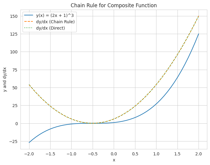
Symbolic Calculation:
y(u) = u**3
u(x) = 2*x + 1
y(x) = f(g(x)) = (2*x + 1)**3
dy/du = 3*u**2
du/dx = 2
dy/dx (chain rule) = 6*(2*x + 1)**2
dy/dx (direct) = 6*(2*x + 1)**2
- We use the `sympy` library to perform symbolic differentiation of a composite function. This clearly shows the application of the chain rule in mathematical terms.
- We also provide an optional numerical visualization by plotting the composite function and its derivative (calculated both directly and using the chain rule), demonstrating that both methods yield the same result.
To an AI/ML engineer
The chain rule is the mathematical backbone of the backpropagation algorithm, which is used to efficiently compute the gradients of the loss function with respect to the weights of a neural network during training.
Neural Networks as Composite Functions: A neural network is essentially a complex composition of many functions (layers). Each layer performs a transformation on its input (weighted sum and activation function), and the output of one layer becomes the input of the next. The final output of the network is a function of all the weights and biases in the network.
Goal: Gradient of the Loss: To train the network using gradient descent (or its variants), we need to calculate the gradient of the loss function $J$ with respect to each weight $w$ in the network, $\frac{∂J}{∂w}$.
Applying the Chain Rule: Because the loss depends on the network’s output, which depends on the activations of the final layer, which depend on the weights of that layer, and so on, we need to use the chain rule to “backpropagate” the gradient of the loss through the network.
Consider a simple case: Loss $J$ depends on the output $y$ of a neuron, and $y$ depends on the weight $w$ and input $x$ through some activation function $σ(wx+b)$. The chain rule allows us to write:
\[\frac{∂J}{∂w}=\frac{∂J}{∂y}⋅\frac{∂y}{∂(wx+b)}⋅\frac{∂(wx+b)}{∂w}\]This shows how the gradient of the loss with respect to the weight w is calculated by multiplying the gradients of the subsequent functions in the chain.
Efficiency of Backpropagation: Backpropagation efficiently computes these gradients layer by layer, avoiding redundant calculations. It calculates the gradient of the loss with respect to the outputs of each layer and then uses these gradients to compute the gradients with respect to the weights and biases of that layer, working backward from the output layer to the input layer.
Complex Architectures: The chain rule extends naturally to more complex network architectures, including convolutional neural networks (CNNs) and recurrent neural networks (RNNs), allowing for the computation of gradients through convolutional layers, pooling layers, and recurrent connections.
1
2
3
4
5
6
7
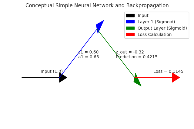
Conceptual Backpropagation:
Prediction: 0.4215
Loss: 0.1145
Gradient of Loss w.r.t. weight1: 0.0214
- We provide a conceptual implementation of the forward and backward passes in a very simple neural network with one hidden layer.
- We manually calculate the gradient of the loss with respect to one of the weights using the chain rule, demonstrating how the error signal is propagated backward through the network.
- A simple diagram illustrates the flow of information in the network and hints at the backward propagation of gradients.
The intuition for what backprop is
To a 5-year old
Imagine you have a big team of toy sorters, and they’re trying to guess if a toy is a car or a truck.
First Sorter: The first sorter looks at the toy’s color and says, “Hmm, it’s red, so maybe it’s a car.” But sometimes red toys are trucks too!
Second Sorter: The second sorter then looks at the number of wheels and says, “It has four wheels, so it’s definitely a car!” But some trucks also have four wheels.
Final Guesser: The final guesser listens to both sorters and makes the final decision: “Okay, based on color and wheels, I think it’s a car!”
Oops! Wrong Guess: But sometimes, the final guesser is wrong! The toy was actually a truck.
Backpropagation (Telling the Sorters They Were a Little Off): Now, we need to teach the sorters to get better. Backpropagation is like going back to each sorter and saying, “Hey, final guesser was wrong. Your clue was a little misleading. Maybe red doesn’t always mean car, and four wheels doesn’t always mean car.”
Learning: The sorters then learn to adjust their thinking a little bit. Maybe the first sorter will think “red” is now a slightly weaker clue for “car,” and the second sorter will think “four wheels” is also a slightly weaker clue.
By going back and telling each sorter how much their clue contributed to the wrong guess, they can all learn to make better guesses together next time!
To an undergraduate student
Imagine training a neural network to classify images. The network makes a prediction, and we compare it to the actual label using a loss function (which tells us how wrong the network was).
The Problem: We want to adjust the network’s internal parameters (weights and biases) to reduce this loss.
The Network as a Chain of Functions: A neural network is a series of interconnected layers, each performing a mathematical operation on the input it receives. The output of one layer becomes the input of the next. This creates a complex composite function mapping the input image to the final prediction.
Backpropagation (Propagating the Error): Backpropagation is an algorithm that efficiently computes the gradient of the loss function with respect to each weight in the network. It does this by using the chain rule of calculus to propagate the error signal backward through the network, layer by layer.
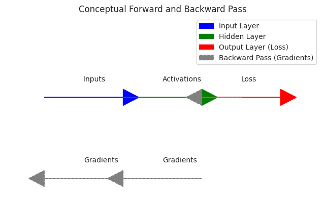
How it Works:
Forward Pass: The input data flows through the network, and a prediction is made. The loss is calculated at the output layer.
Backward Pass: The gradient of the loss with respect to the output layer’s activations is calculated. Then, this gradient is used to calculate the gradient with respect to the weights and biases of the output layer. This process is repeated, moving backward through the network. The gradient at each layer tells us how much a change in the weights and biases of that layer would affect the final loss.
Why is it Intuitive? Think of the error signal originating at the output. We want to understand how much each parameter in the network contributed to this error. Backpropagation allows us to distribute this “blame” or “responsibility” back through the network. Parameters that had a larger impact on the error will have larger gradients.
Using the Gradients for Learning: These gradients are then used by optimization algorithms like gradient descent to update the weights and biases in the direction that reduces the loss. The learning is iterative: forward pass to see the error, backward pass to calculate how to adjust the parameters, and then update the parameters.
To an AI/ML engineer
Backpropagation is the workhorse of modern deep learning, enabling the efficient training of complex neural networks. The intuition lies in its computational efficiency in calculating gradients across a deep and interconnected computational graph.
Computational Graph: A neural network can be viewed as a directed acyclic graph (DAG) where nodes represent operations (layers, activation functions) and edges represent the flow of data.
The Challenge of Direct Differentiation: Directly calculating the gradient of the loss with respect to every parameter in a deep network would be computationally very expensive, involving redundant calculations of intermediate derivatives.
Backpropagation (Leveraging the Chain Rule and Dynamic Programming): Backpropagation solves this by using a dynamic programming approach combined with the chain rule. It performs two passes:
Forward Pass: Computes the output of each node in the graph. The intermediate activations are stored for use in the backward pass.
Backward Pass: Computes the gradient of the loss with respect to each node’s output, starting from the output layer and moving backward. The key insight is that the gradient with respect to a node’s input can be efficiently computed using the gradient with respect to its output and the local gradient of the operation performed by the node.
Local Gradients: Each operation in the network (e.g., matrix multiplication, activation function) has a well-defined local gradient with respect to its inputs. The chain rule allows us to combine these local gradients to obtain the global gradient of the loss with respect to any parameter.
Intuition for Efficiency: Instead of recalculating the same intermediate gradients multiple times, backpropagation computes them once and reuses them. This significantly reduces the computational cost, making training deep networks feasible.
Gradient Flow and Vanishing/Exploding Gradients: Understanding backpropagation also provides intuition for issues like vanishing and exploding gradients. If the local gradients at each layer are consistently very small or very large, the gradients propagated backward can become exponentially small or large, hindering learning in deep networks.
Automatic Differentiation Frameworks: Modern deep learning frameworks (like TensorFlow and PyTorch) automate the process of backpropagation using techniques like automatic differentiation. Engineers don’t need to manually derive and implement the backward pass for every new layer; the framework handles it by tracking the operations performed during the forward pass.
1
2
3
4
5
6
7
8
9
10
11
12
13
14
15
16
17
18
19
20
21
22
23
24
25
26
27
28
Conceptual Backpropagation in a Layer:
Inputs (batch x features):
[[0.37 0.95 0.73 0.6 ]
[0.16 0.16 0.06 0.87]]

Weights (features x neurons):
[[0.6 0.71 0.02]
[0.97 0.83 0.21]
[0.18 0.18 0.3 ]
[0.52 0.43 0.29]]

Activations (batch x neurons):
[[0.98 0.92 0.72]
[0.87 0.64 0.54]]

Gradient of Loss w.r.t. Activations:
[[0.37 0.46 0.79]
[0.2 0.51 0.59]]

Gradient of Loss w.r.t. Weights:
[[0.01 0.04 0.1 ]
[0.01 0.06 0.21]
[0.01 0.03 0.15]
[0.03 0.15 0.3 ]]

Gradient of Loss w.r.t. Biases:
[0.03 0.19 0.4 ]
Miscellenous
Try out: Colab Notebook